Excel has a lot of functions which make your life easier. One such feature is Goal Seek. It can be used to help you speed up your calculations. Goal Seek is part of a suite of commands sometimes called what-if analysis tools. When you know the desired result of a single formula but not the input value of the formula needed to determine the result, you can use the Goal Seek feature.
When goal seeking, Microsoft Excel varies the value in one specific cell until a formula that’s dependent on that cell returns the result you want. I am explaining it by taking an example, Say, You’ve got a fixed amount of your monthly salary that can go towards your loan payment and are now wondering which interest rate will best suit you. Here is how you can solve it using Goal Seek.
STEP 1: Create a table
The use of estimate amounts for calculations will result in an inaccurate result. Hence, the first step
to answer a loan-related query is to get accurate values for all the factors revolving around the loan
scheme. Before initiating the goal seek feature, enter these values into a new worksheet.
-
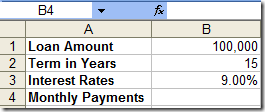
Enter the factors “Loan Amount”, “Term in Years”, “Interest Rate”, and “Monthly Payment” in
cells “A1”, “A2”,”A3”, and “A4”. -
In cell “B1”, enter the loan amount that you need to pay back to the lender; for example, the total
loan amount is 100,000. -
In cell “B2”, enter the number of years it would take to complete the loan payment. For example, the term allocated to complete the loan payment is 15 years.
-
Then in cell “B3”, enter the estimated interest rate that is likely to result in a value close to your fixed monthly budget. For example, on considering the previous values, you can estimate an interest rate of 9% if you have a monthly budget of 900.

STEP 2: Enter the PMT function
In order to use the Goal Seek tool effectively, the base model must be set up in your worksheet with the formula already in place and working.
-
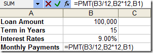
In the cell “B4”, enter the formula “=PMT(B3/12,B2*12,B1)” to calculate the monthly payment. (Refer to tip “Access the PMT function Quickly”).
-
You see that a monthly payment of “1,014.27” is calculated

The PMT function calculates monthly payments based on the loan amount, interest rate, and length of time it will take to pay back the money. The syntax for the PMT function is PMT (interest rate per period, number of payments, and loan amount )
STEP 3: Use the Goal Seek tool
Goal Seek can be used when you know the result of a formula but not the input value required by the
formula to decide the resulting reverse calculation. You can change the value of a specified cell until
the formula that is dependent on the changed cell returns the result you want.
-
Go to “Tools > Goal seek”.
-
In the “Goal seek” dialog box that opens up, click on the cell containing the formula to enter it into the “set cell” field
-
In the field “To value”, enter the value that you need to arrive at. For example, you have a target value of 900 as the fixed monthly payment you can afford. Enter this value as “-900”.
-
Then, in the field “By changing cell”, enter the cell reference of the value that needs to be changed. For example, cell B3 needs to be clicked in order to change the interest rate. Click OK
-
The “Goal seek status” dialog box appears with the information of the cell reference, the “Target Value” and the “current Value” that Goal Seek has arrived upon. Click OK
