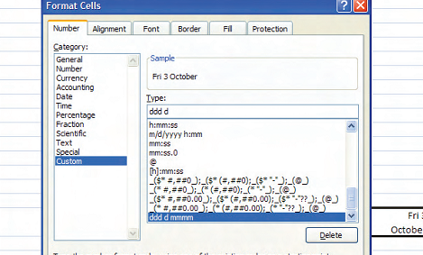
Formatting cells to suit your requirement in Excel is one of the easiest tasks to perform. Excel is flexible enough to let you customize formats to suit your needs as well. But what if you require two lined custom formats in Excel?
You can use the wrap text feature of Excel but that depends on the column width and text length. You can use the [Alt] + [Enter] break key, but it does not work with formats. What if you need a format with the day and date on top followed by the month?

You can maintain consistency by creating a multi-line custom format with the help of this simple tip. To do so just carry out the following steps:
-
Select the cell to which the format is to be applied.
-
Click the “Home” tab. Click the small arrow near the “Numbers” group.
-
The “Number” tab of the “Format Cells” dialog box appears.
-
Under the “Category” list, select the “Custom” option.
-
In the “Type” text box, type “ddd d” without the quotes.
-
Press the [Alt] key and type “0010” from the numeric keypad.
-
The cursor jumps to the next line.
-
Although it is not visible, Type “mmmm” without the quotes.
-
Next, click the “Alignment” tab.
-
Check the “Wrap Text” option.
You can try this tip to make your custom formatted cells in multiple lines. Also check out our previous Microsoft Excel Tips.
